EV telemetry: what the battery is really doing

A battery current reading is two measurements in one sign. Positive means the pack is supplying power; negative means the car is recovering energy while it brakes or coasts. That single signed number is what a range estimate, a thermal model or an energy dashboard actually needs, and it is what this project estimates from signals available at the same instant: speed, acceleration, pedal travel, road grade, and the ECO / air-conditioning states.

It began as the term project for Python for Engineers at the Turkish-German University. The brief was open-ended, so I treated it as a small engineering study rather than a plot collection: clean the data honestly, state a physical model with its assumptions, compare it with a learned model and a mean baseline, and analyse where each one fails.

The question, stated precisely

Can CUR — battery current in ampere, signed, including regenerative braking — be estimated from simultaneous vehicle signals only? Not forecast: every feature is measured at the same timestamp as the target. The test set is the latest 20 % of the recorded time, so the score measures performance on unseen drivers and an unseen day.

That choice matters. A random split would let the model memorise the route and the driver, and it would look far better than it is.

The data are not clean, and that is part of the story

The dataset is public: nine trips over the same ~76 km route in Brazil, October 2023, 24,277 rows at roughly 2 s sampling. It is also messier than its description suggests:

pack voltage qualityphoto

• The file is shuffled. Rows from all trips are interleaved; sorting per trip is the first operation.
• 97 timestamps cannot be trusted. Impossible components (month 49, hour 83) or stamps contradicting the recording order are dropped, because there is no honest way to place them in time.
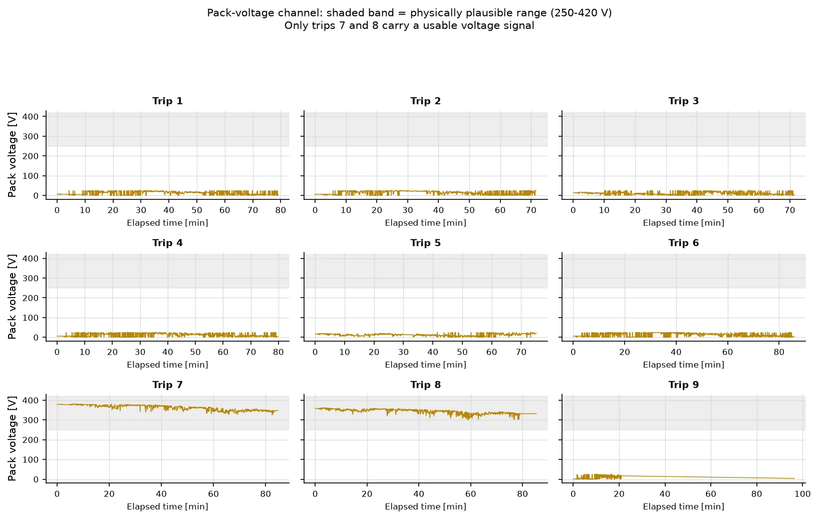
• Corrupt channels are flagged, not deleted. Pack voltage is outside 250–420 V on 18,049 rows; altitude has four zero sentinels; 21 GPS fixes fall outside Brazil. Those rows still carry valid speed and current, so they stay, with vol_valid, alt_missing and gps_valid flags.
• The accelerometer is unusable as acceleration. AX has a per-trip offset between −0.1 and +3.1 m/s² and correlates with differentiated speed at only r = 0.14. The pipeline uses dSPD/dt instead, and documents why.

The cleaning report is generated, not hand-written: every count in the project comes from the same code path that produced the figures.

A physical model first

The reference model is a longitudinal power balance at the pack:

I = [ m·a·v + ½·ρ·C_d·A·v³ + m·g·sin(θ)·v + C_rr·m·g·v ] / (η·V_nom)
    + (P_base + P_air·AIR) / V_nom

Dividing by the nominal pack voltage makes the equation linear in six coefficients — apparent mass, aerodynamic drag, grade force, rolling resistance, base load and air-conditioning load — so it can be calibrated by ordinary least squares on the training rows alone. Grade comes from altitude and odometer over a trailing ~30 s window; it is causal, not a centred smoothing.

The fitted coefficients are converted back into engineering quantities, which is where the model earns or loses trust. Two independent estimates of vehicle mass — one from traction, one from grade — agree within 10 % (873 kg and 959 kg). Both sit about 40 % below the published 1,535 kg kerb mass, most plausibly because a 2 s finite difference smooths acceleration peaks and one efficiency cannot describe traction and regeneration at once. That is a reported limitation, not a number I tuned away.

Then a learned model, and a baseline that keeps everyone honest

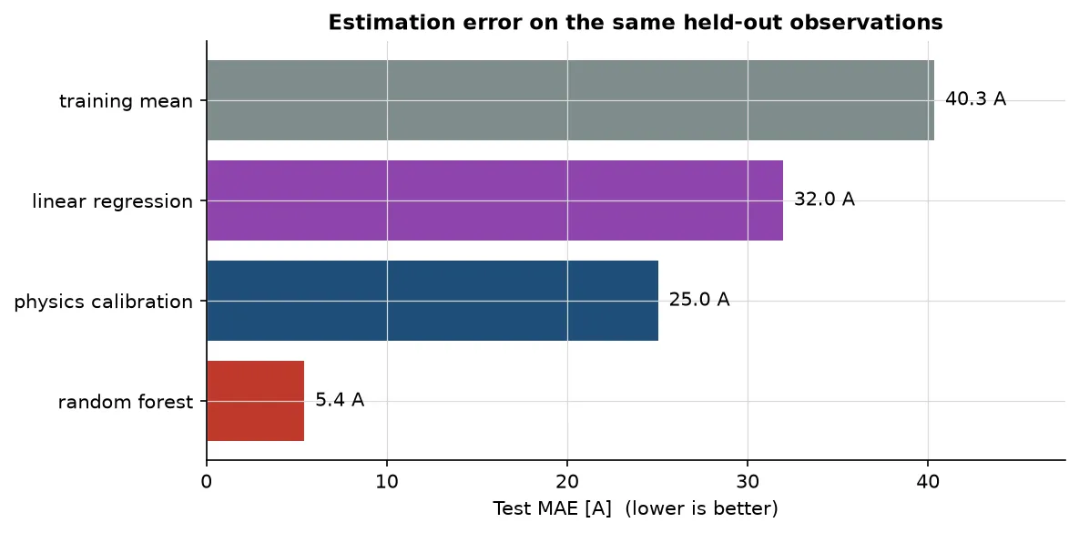
Four methods are scored on the same held-out rows. The Random Forest is tuned with time-series cross-validation inside the training set; no test row influences the imputer or the hyper-parameters. The optional linear regression on speed and acceleration is the simple reference the brief allowed.

Model	Test MAE	RMSE	Bias	R²
Training mean (baseline)	40.35 A	54.58	−2.84	−0.003
Linear: speed + acceleration	31.96 A	43.94	−2.62	0.350
Calibrated physics	25.03 A	36.05	−0.47	0.562
Random Forest	5.43 A	9.43	−0.47	0.970

test MAEphoto

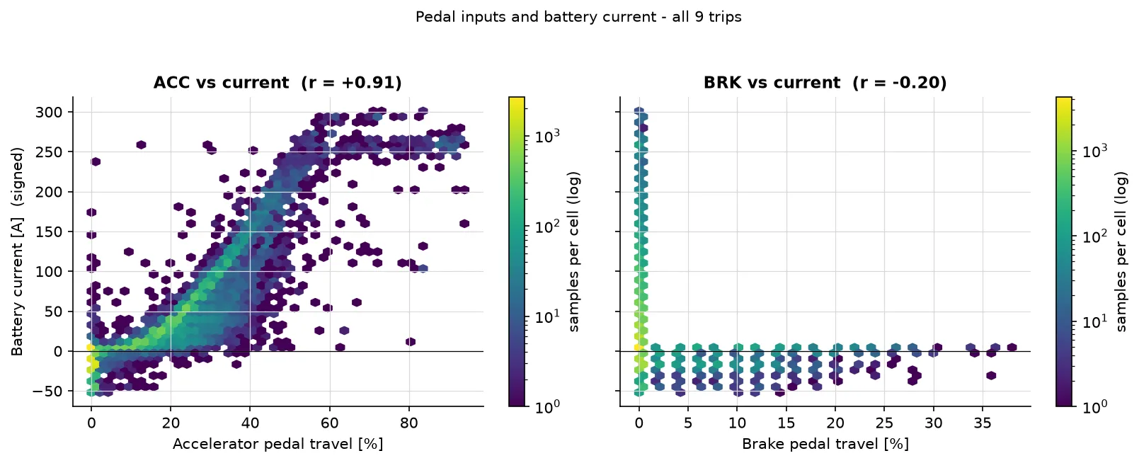
The gap has a clear cause. The accelerator pedal alone correlates with current at r = +0.91, and 90 % of the forest’s feature importance lands on ACC. The forest is, to a large extent, a learned pedal-to-current map of this particular vehicle. That is a legitimate simultaneous signal, but it is also why the physics model is the one that would transfer to another EV, while the forest is tied to this pedal calibration.

pedal responsephoto

Where the errors live

error analysisphoto

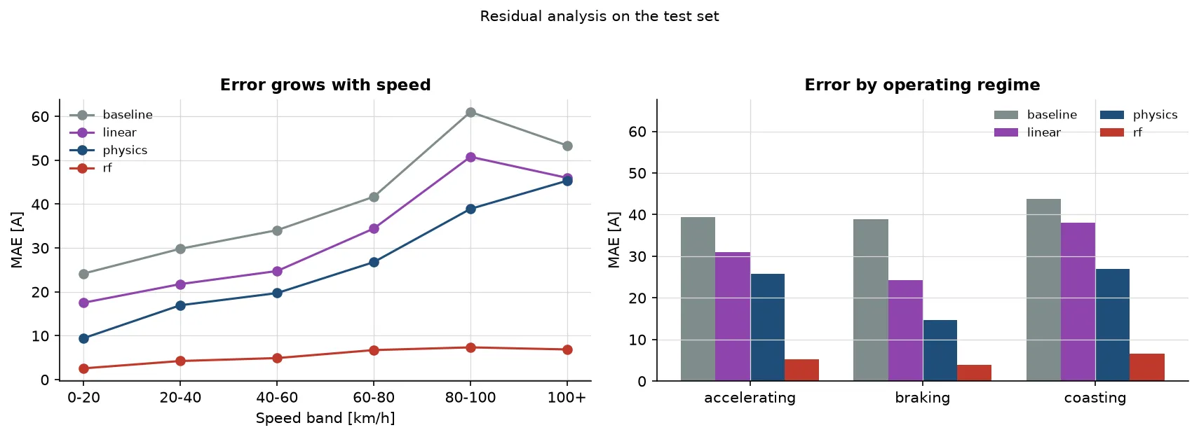
The pattern is informative rather than decorative:

• The baseline has a −36 A bias above 80 km/h and −29 A uphill. It predicts the average of a mostly low-demand dataset and cannot follow demand.
• The physics model is best while braking (14.6 A), where the recovery term is proportional to speed and dominates, and worst above 80 km/h (39–45 A), where aerodynamic and efficiency assumptions matter most.
• The forest stays between 3.9 A (braking) and 6.5 A (coasting) per regime. Its largest remaining bias is about −3.5 A at 80–100 km/h.

A second split holds out the last 20 % of every trip, putting all nine drivers in the test set. The ranking does not change (forest 6.2 A, physics 27.2 A, linear 33.2 A, baseline 38.5 A), so the result is not an artefact of which trips happen to fall after the global cut.

The ECO-mode trap

Trip 4 switches economy mode on and off four times: same car, same route, same driver. The raw numbers look like a clean result — and they are wrong. ECO-on windows also contain twice the accelerator pedal (27 % versus 12 %) and sit on slightly uphill sections (+2.2 % versus −1.2 % grade). Raw current is therefore higher with ECO on: 49.5 A versus 19.7 A.

ECO experimentphoto

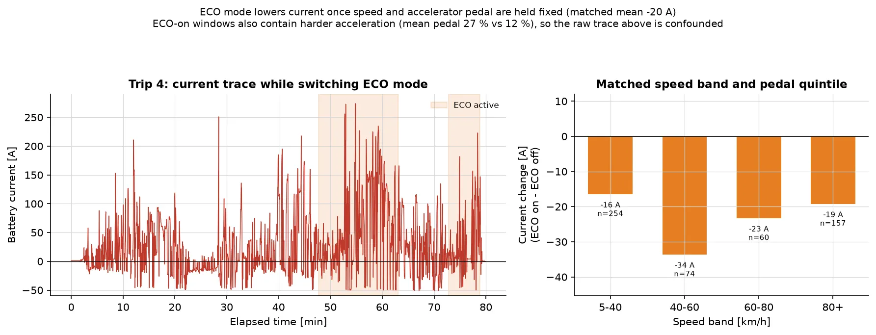
Comparing only samples in the same speed band and the same pedal quintile reverses the sign: ECO-on is 16–34 A lower in every band, with a matched average of −20 A (a regression that also controls for grade gives ≈ −15 A). The mode does save current; the raw comparison was measuring the driver’s right foot.

That reframing is the part of the project I would keep in any future analysis. Observational data rarely gives you a clean experiment, and matching is often the difference between a finding and a plausible-looking artefact.

What I would change next

• More drivers and more days. The global test set is two drivers on one day; the per-trip check mitigates but does not remove that limitation.
• Separate charge and discharge efficiencies, and a shorter acceleration window, to see whether the fitted mass moves toward the published kerb mass.
• A transfer test. Train the pedal map on one vehicle and apply it to another; my expectation is that the physics model degrades gracefully and the forest does not.
• A proper state-of-charge model. Current integrates to charge, so the natural next step is a small battery model rather than a single-step estimate.

The code, the executed notebook, the data-quality report and all figures are in the repository. The raw dataset is GPL-3.0 and is not redistributed; the pipeline downloads it from Kaggle and rebuilds everything else.

Code and notebook on GitHub →