Ground-analysis rover

The interesting part of this rover isn’t that it drives. It’s that it builds an opinion about the ground underneath it: it turns a stream of noisy, bare-metal sensor readings into a geo-referenced map of where the road is rough, where it dips, and where it bumps. This is the full path from sensor to state to meaning, built for a real course deliverable and then built a second time in simulation to prove it out.

photo: rover top-downphoto

The problem

This started as a smart-city question. Cities find potholes and broken pavement with expensive survey vehicles or by hand. Could a cheap mobile robot do the same job automatically and tag every defect with a coordinate?

Most terrain mapping leans on cameras or LiDAR: exteroceptive sensing that looks ahead at the world. That breaks down exactly where it matters, in dust, glare, low light, or over featureless ground. Proprioceptive terrain analysis takes the opposite stance. Instead of asking “what does the ground look like?”, it asks “what does the ground do to me as I move across it?”

Vertical acceleration and tilt are the two answers that change how a robot should drive. A sharp jolt up means a bump, a drop means a pothole, sustained tilt means slope. All of it is recoverable from motion alone, if you can read the robot’s state precisely enough and trust your timing.

Two parallel builds

The project ships as two working systems, and the distinction matters because each one carries a different half of the story:

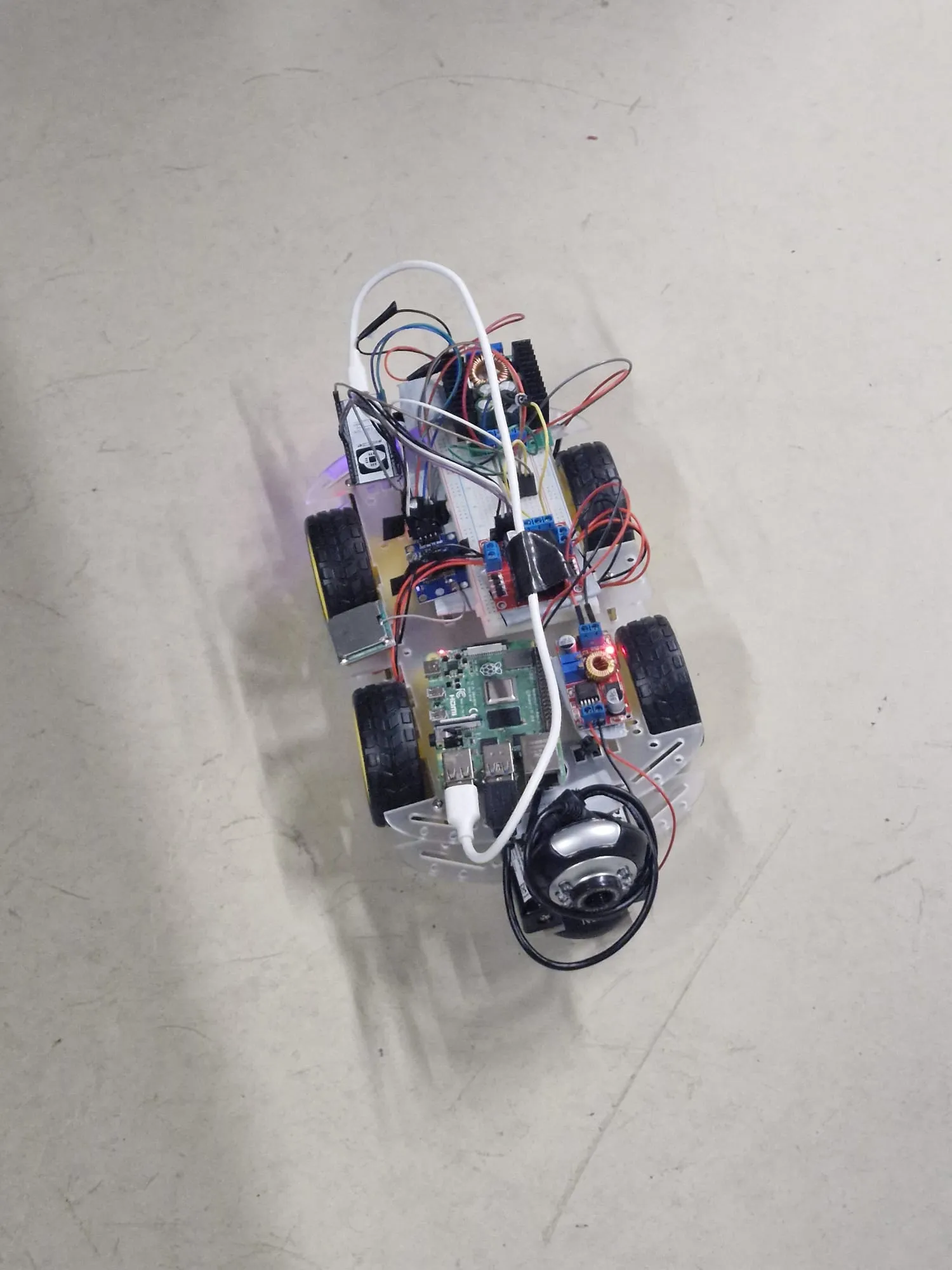
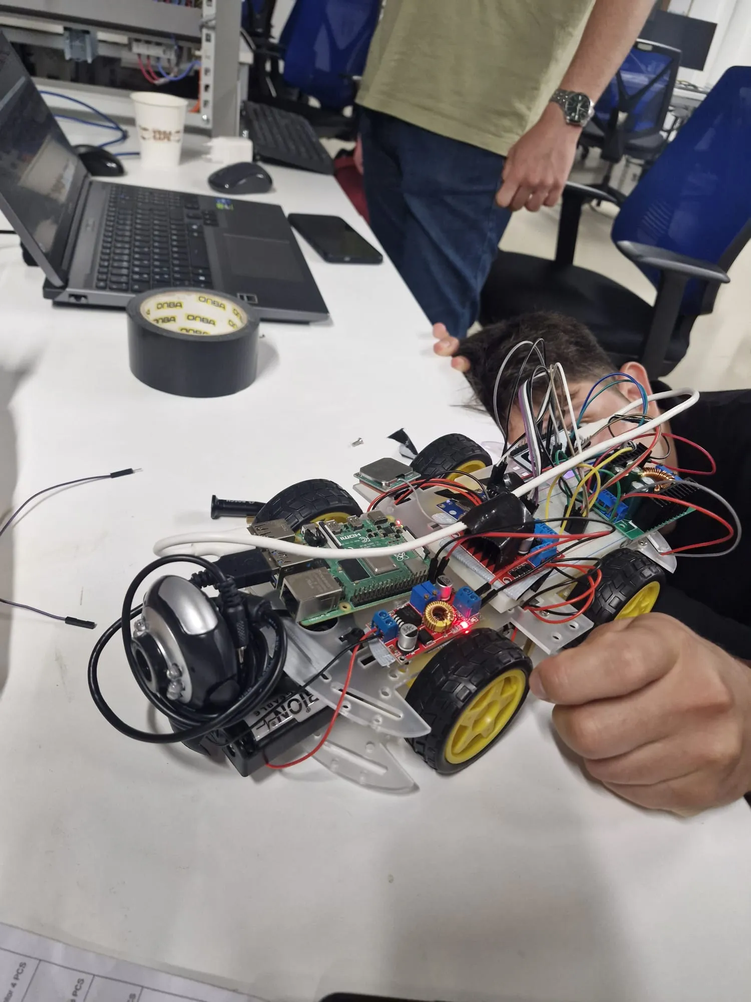
1. The physical robot. An ESP32 running FreeRTOS and micro-ROS for the hard-real-time layer, a Raspberry Pi 4 running ROS 2 Jazzy for the application layer, joined over a USB serial micro-ROS bridge. It classifies the ground live with a threshold algorithm and plots every event on a browser dashboard.
2. The simulation digital twin (rover_ws). ROS 2 Jazzy + Gazebo Harmonic, modelled on the real kit’s dimensions. This is where the heavier perception lives: a dual-EKF localization stack with GPS fusion, and a proprioceptive terrain heatmap that scores slope and roughness into an occupancy grid.

The hardware proves it works in the real world with real noise. The twin is where the estimator and the mapping get to be ambitious without fighting a brownout at the same time.

The physical robot

The architecture is split across two compute domains on purpose: a microcontroller close to the sensors doing hard-real-time work, and a Linux SBC running the ROS 2 graph. micro-ROS is the bridge that makes the ESP32 a first-class citizen on the same DDS network as the Pi.

architecture diagrampending

architecture diagramasset placeholder

This separation is the whole point. Timing-critical sampling and the motor loop live on bare metal, where jitter is measured in microseconds. Everything that benefits from a real operating system, the camera, the web stack, the map, lives on the Pi.

photo: hardware detailphoto

Sensor layer

The ESP32 reads an MPU6050 IMU over I2C and a NEO-6M GPS over a second UART. The IMU is fast and drifts, the GPS is slow and absolute and arrives late, and neither is usable alone. The firmware samples the IMU at 50 Hz, timestamps honestly using a synced session clock, and ships everything north over micro-ROS as standard sensor_msgs/Imu and sensor_msgs/NavSatFix messages.

The classification itself is a deliberately simple, calibrated threshold rule. The course required a real logical decision algorithm, and a transparent one beats a black box you cannot defend:

// Ground classification from vertical acceleration
const float G = 9.81f;
const float TH_BUMP    = 1.8f * G;   // sharp jolt up
const float TH_POTHOLE = 0.3f * G;   // momentary free-fall

if      (az > TH_BUMP)    event = "ERHEBUNG";    // bump
else if (az < TH_POTHOLE) event = "SCHLAGLOCH";  // pothole
else                      event = "EBEN";        // flat

Every non-flat event is stamped with the current GPS fix, which is what turns a stream of accelerations into a map a city could act on.

The dashboard

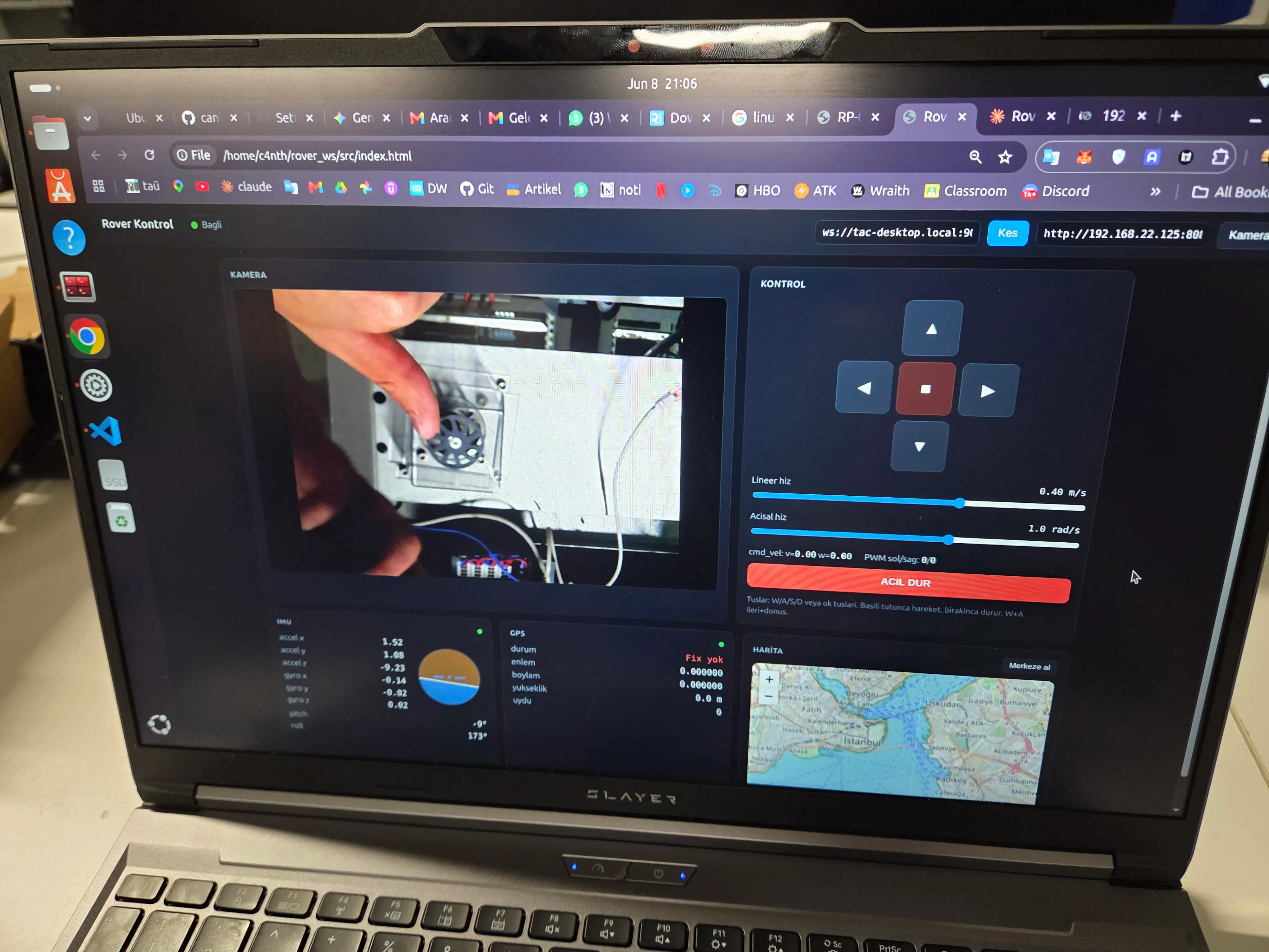
The payoff on the hardware side is a live browser dashboard served off the Pi: teleop controls, the camera as an MJPEG stream, raw IMU and GPS telemetry, and a Leaflet map that drops a marker wherever the robot is. Drive it around, watch the fix lock on, and the map fills in.

photo: live dashboardphoto

The simulation digital twin

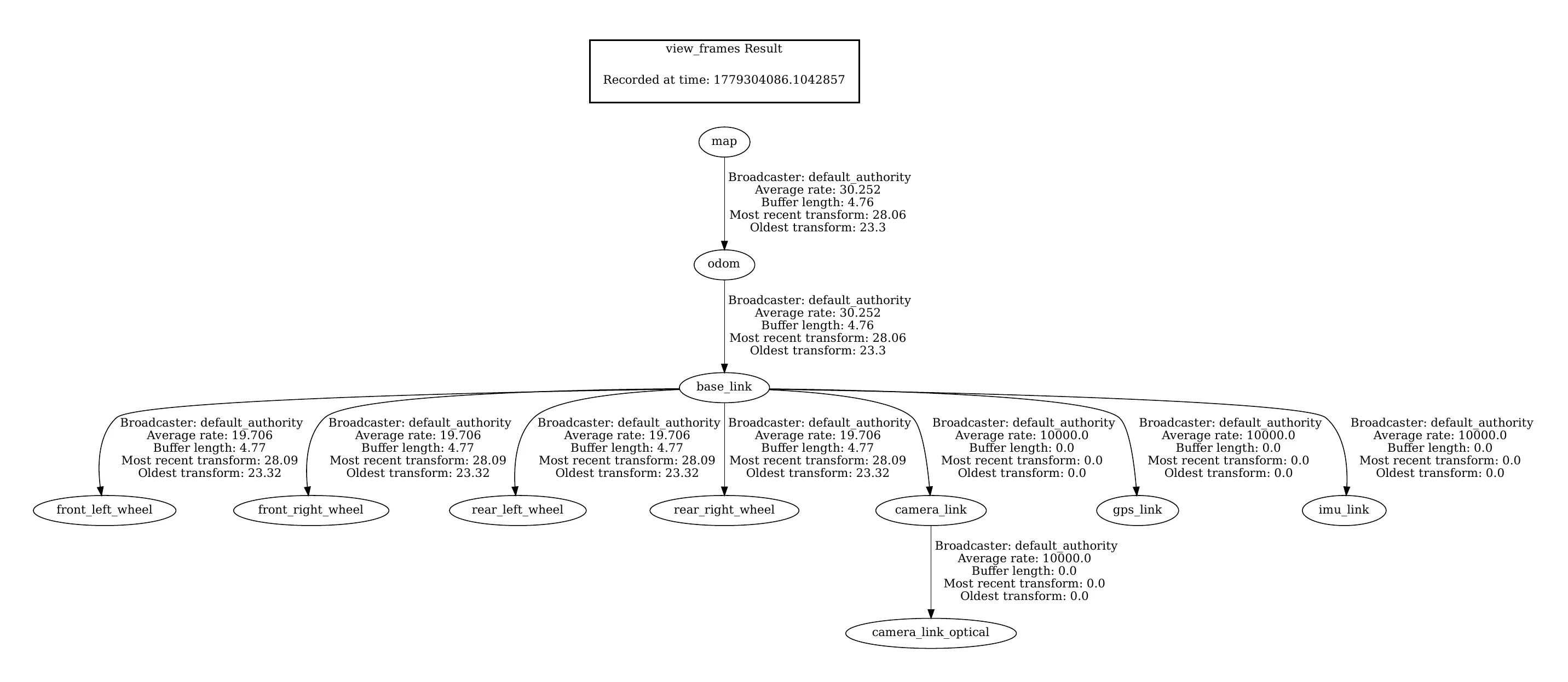
The twin mirrors the physical kit (25.5 x 15 cm chassis, 65 mm wheels, 4-wheel skid-steer) inside Gazebo Harmonic, and it is where the perception stack gets to be honest about state. The whole thing comes up with one command:

ros2 launch rover_bringup bringup_demo.launch.py world:=terrain_world.sdf

That brings up the sim, a ros2_control differential-drive controller with skid-steer slip compensation, the localization stack and the mapping node, all visualised in RViz.

State layer: the EKF

This is the seam I care about most. A dual Extended Kalman Filter setup from robot_localization fuses the high-rate IMU with low-rate GPS: a local EKF in the odom frame for smooth, continuous motion, and a global EKF in the map frame that folds in GPS through navsat_transform for absolute drift correction. The EKF’s job is to hold a belief about where the robot is and how it is oriented, and to update that belief sensibly every time a new, imperfect measurement arrives.

The honest version: getting an EKF to converge and stay converged is mostly about trusting the right sensor at the right moment, tuning the process and measurement noise so the filter leans on GPS for absolute correction and on the IMU for everything fast in between.

tf frame treephoto

// EKF core: predict on fast IMU, correct on slow GPS
state = f(state, imu, dt);             // motion model
P     = F * P * F.t() + Q;            // grow uncertainty
if (gps.fresh()) {                    // absolute, low rate
  K     = P * H.t() * (H * P * H.t() + R).inverse();
  state = state + K * (gps.z - h(state));
  P     = (I - K * H) * P;            // shrink uncertainty
}

Meaning layer: the heatmap

State becomes meaning in terrain_heatmap_node. It subscribes to the IMU at 100 Hz and odometry at 50 Hz, and writes two 200 x 200 occupancy grids (20 cm cells over a 40 x 40 m area):

• Slope falls out of gravity’s direction in the IMU frame, smoothed with an IIR low-pass filter and normalized to a 25 degree full scale.
• Roughness falls out of the high-frequency vertical-acceleration energy an IIR high-pass filter isolates, normalized to 5 m/s² full scale.

Two details make it trustworthy. Each cell tracks its peak, not its average, so a single sharp pothole never gets averaged into invisibility. And outliers (slopes past 40 degrees, roughness past 10 m/s²) are rejected outright. The output is not a number on a dashboard, it is a field: a map where every cell carries how steep and how rough that ground is. That is the world model.

rviz capturepending

rviz captureasset placeholder

What I owned

I led perception and the embedded backbone in a five-person team. Concretely, that meant the ESP32 firmware and sensor layer, the micro-ROS integration that joined it to the ROS 2 graph, the threshold classifier and GPS tagging on the hardware, and on the twin the EKF localization and the slope / roughness mapping that turned state into the heatmap. Teammates owned the mechanical platform, power wiring, and parts of the dashboard front end.

I’m naming scope deliberately, because “I built a rover” usually hides who built what. I built the path from the sensor to the map.

What broke / what I’d change

The part most portfolios skip. A few honest ones, all of which are documented in the project’s own engineering log:

• The whole system browned out before it ever drove. Thin shared-ground wiring and a split 5 V supply caused resets under motor load. The fix was a single star-point ground, thick short power leads, and isolating the dirty motor rail from a clean sensor rail. Embedded power is not an afterthought, it is the platform.
• A copy-paste bug cost an evening. ROS C type names use double underscores (sensor_msgs__msg__Imu), and pasting firmware between editors silently collapsed them to single underscores, breaking every build. The fix was embarrassing and real: keep the code in a file, stop pasting it.
• GPS indoors and near structures is a different animal than GPS in an open field. A NEO-6M cold start under a roof takes minutes, so we learned to watch the satellite count and trust the fix only once it earned it.
• The simulation’s hardest wall was physics, not perception. Skid-steer in Gazebo wanted to flip; getting stable behaviour meant working through friction models and switching physics engines, not tuning the mapping.
• Next time: I’d feed the heatmap from the EKF pose instead of ground-truth odometry in sim, add wheel odometry as a third filter input, and treat estimator tuning as a logged experiment instead of a feel.

That’s the real engineering: not that it worked, but knowing exactly where and why it didn’t.